
| 일 | 월 | 화 | 수 | 목 | 금 | 토 |
|---|---|---|---|---|---|---|
| 1 | 2 | 3 | 4 | |||
| 5 | 6 | 7 | 8 | 9 | 10 | 11 |
| 12 | 13 | 14 | 15 | 16 | 17 | 18 |
| 19 | 20 | 21 | 22 | 23 | 24 | 25 |
| 26 | 27 | 28 | 29 | 30 |
- machinelearning
- 파이썬
- 코테
- 전처리
- 연산자
- code
- 머신러닝
- 데이터분석
- pandas
- mysql
- 데이터사이언스
- 데이터과학
- 캐글
- 아마존
- Python
- dataframe
- 데이터전처리
- kaggle
- SQL
- numpy
- 시각화
- 불리언
- 프로그래머스
- data science
- get_dummies
- 코딩테스트
- 데이터 전처리
- Data Analysis
- 데이터구조
- EDA
- Today
- Total
Road to Data Scientist
[Spaceship Titanic] 1st : XGBooster, Light GBM, Logistic Regression, Decision Tree, Random Forest - part1 : 데이터 불러오기& 데이터 탐색 본문
[Spaceship Titanic] 1st : XGBooster, Light GBM, Logistic Regression, Decision Tree, Random Forest - part1 : 데이터 불러오기& 데이터 탐색
ShazelP 2024. 4. 12. 23:05Kaggle Competition : Spaceship Titanic
Spaceship Titanic | Kaggle
www.kaggle.com
Kaggle의 기본 예측 데이터셋인 "Titanic 생존자 예측" 과 같이 "우주선 탑승객 예측"을 하는 기본 대회 데이터셋으로, 우주선 탑승객의 환승여부를 예측하는 것을 목표로 함.
1. SET UP
- Import library: 데이터 탐색, 엔지니어링, 시각화, 머신러닝 등등을 위한 기본 라이브러리 다운
import numpy as np
import pandas as pd
#for visualization(그래프 그리기 위한 라이브러리 다운로드)
import matplotlib.pyplot as plt
import seaborn as sns
2. LOAD DATA
- 제공된 데이터를 불러오고 기초적인 탐색을 위한 단계
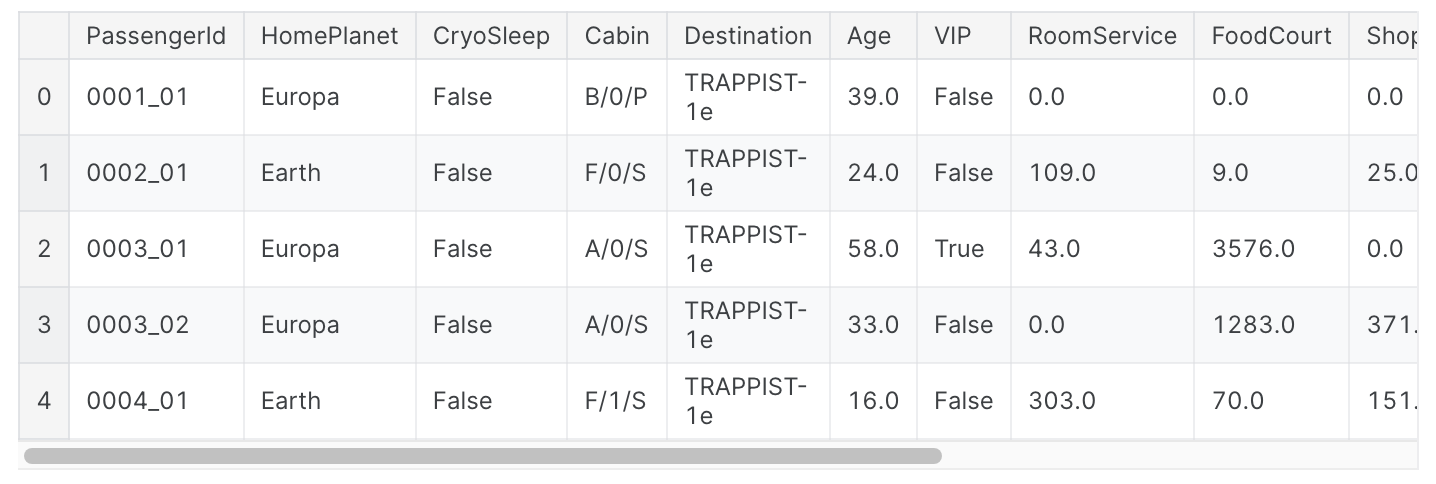
train 데이터 불러오기
data = pd.read_csv("/kaggle/input/spaceship-titanic/train.csv")
data.head()
#output
test 데이터 불러오기
test = pd.read_csv("/kaggle/input/spaceship-titanic/test.csv")
test.head()
#output

train 데이터 크기 확인
data.shape#output
(8693, 14)
- 총 (8,693 열 x 14행)으로 구성되어 있음
train 데이터 기초통계 확인
#describe all columns
data.describe(include='all')
#output

Missing Values 결측치 확인
#count null (null 값 찾기)
data.isna().sum()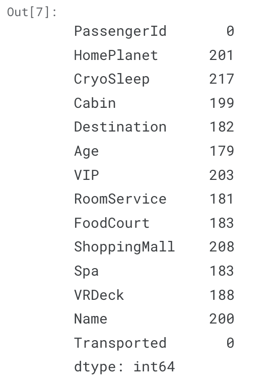
- PassengerId, Transported 를 제외한 모든 열이 결측치를 갖고 있음 --> 어떻게 처리할 것인지? 추후 고민
3. EDA & VISUALIZATION
- 시각화(그래프)를 이용한 데이터 속성 확인하기
HomePlanet Column
#HomePlanet

fig, axs = plt.subplots(figsize=(10,10),nrows=2) # 두 열로 이루어진 각각 그래프
#첫번째 그래프: HomePlanet values 개수 세기
data['HomePlanet'].value_counts().plot(kind='bar', ax=axs[0])
#두번째 그래프: HomePlanet value 개수를 예측해야 하는 Transported 여부로 나누어서 개수 세기
sns.countplot(data=data, x='HomePlanet', hue='Transported',
              order = data['HomePlanet'].value_counts().index, ax=axs[1])

#두 그래프 사이 간격 자동으로 조정
fig.tight_layout()

- Europa와 Mars 출신의 승객이 Transported 하는 경우가 많음
Destination Column
- 위의 그래프와 동일하게 코드 작성
#Destination
fig, axs = plt.subplots(figsize=(10,10),nrows=2)

data['Destination'].value_counts().plot(kind='bar', ax=axs[0])
sns.countplot(data=data, x='Destination', hue='Transported',
              order = data['Destination'].value_counts().index, ax=axs[1])

fig.tight_layout()

- 목적지가 '55 Cancri e', 'PSO J318.5-22' 인 승객이 Transported 하는 경우 많음
Age Column
#Age
#두 개의 열로 이루어진 각각의 그래프
fig, axs = plt.subplots(figsize=(10,10), nrows=2)

#첫번째 그래프: histogram으로 나이대 살펴보기
data['Age'].plot.hist(ax=axs[0])
#두번째 그래프: 나이대와 transported 같이 살펴보기
sns.histplot(x='Age', hue='Transported', data=data, ax=axs[1])

#두 그래프 간격 자동 조정
fig.tight_layout()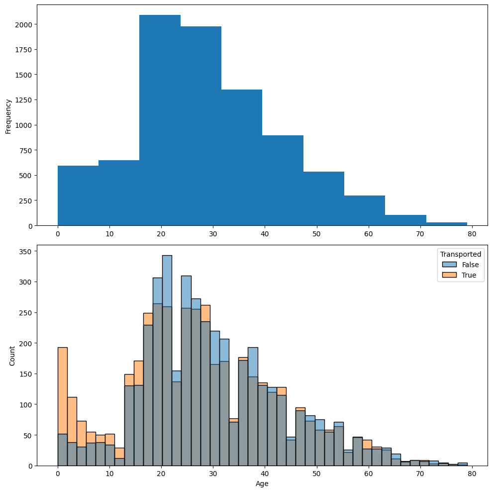
- 나이대별로 transported 경우 다름
Spending Columns
-'RoomService', 'FoodCourt', 'ShoppingMall', 'Spa', 'VRDeck' 의 분포 살펴보기
#Spending on Spaceship
data[['RoomService', 'FoodCourt', 'ShoppingMall', 'Spa', 'VRDeck']].hist(bins=50)
plt.tight_layout()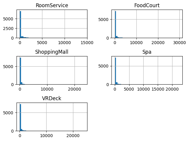
- 대부분의 탑승객 우주선에서 소비 많이 하지 않음
Kaggle 에서 해당 Code 보기
: 아래의 코드에서 머신러닝 모델만 변경하여 적용했습니다.
Spaceship Titanic with Logistic Regression
Explore and run machine learning code with Kaggle Notebooks | Using data from Spaceship Titanic
www.kaggle.com